Back Cover
In a world of AI autopilot, this book teaches you how to take the wheel—by getting to the bottom of things, not just skimming the top.
AI does the work. But do we still understand it? Can we debug, adapt, build from scratch? Or are we now just passengers?
I see it every day— students lost in the basics. Files? Configs? Crashes? Blank stares.
This book brings back the core skills. Not anti-AI but pro-agency. So if you want to build with understanding, read this book.
Totally Real Reviews
"Turns out, the answer wasn’t 'add more layers'."
— Ike Newton, Warden, Royal Mint Systems
"This book is the antidote to the collective amnesia setting in."
— Chuck Babbage, Professor, Cambridge University, UK**
"Finally, a book that dares to whisper what we've all screamed into the void."
— Gracie Hopper, Software Project Manager, US Navy, USA
"Every page is a gentle slap reminding us that AI isn’t magic—it’s math wrapped in marketing."
— Al Turing, Director, Computing, University of Manchestor, UK
About the Author
Tim Menzies (Ph.D. UNSW 1995, ACM Fellow, IEEE Fellow, ASE Fellow) is a globally recognized leader in software engineering research, best known for his pioneering work in data-driven, explainable, and minimal AI for software systems. Over the past two decades, his contributions have redefined defect prediction, effort estimation, and multi-objective optimization, emphasizing transparency and reproducibility.
As the co-creator of the PROMISE repository, Tim helped establish modern empirical software engineering, showing that small, interpretable AI models can outperform larger, more complex ones. Currently, he works as a full Professor in computer science at NC State, USA. He is the director of the Irrational Research lab (mad scientists r'us). His research has earned nearly $20 million in funding from agencies such as NSF, DARPA, and NASA, as well as from private companies like Meta, Microsoft and IBM.
Tim has published over 300 papers, with more than 24,000 citations, and advised 24 Ph.D. students. He is the editor-in-chief of the editor-in-chief of the Automated Software Engineering journal and an associate editor for IEEE TSE. His work continues to shape the future of software engineering, focusing on creating AI tools that are not only intelligent but also fair, transparent, and trustworthy.
For more information, visit http://timm.fyi.
The Forgotten Bits
In this AI-powered age, the tools are dazzling. Code writes itself. Systems configure themselves. Everything is faster, easier, more accessible. And that’s a win—for most. Now, more people than ever can build more things and ship them sooner. That’s democratic. That’s powerful.
But there’s a cost. Surgeons don’t learn by turning their backs on patients and browsing web pages. They learn by reaching in—by touching what they do—so they know where to go when something breaks. Similarly, if you're training to be a software engineer (or working at the edge of research) you can’t just drive the car. You need to know what’s under the hood.
My students struggle with this, all the time.
- They’ve never configured a system from scratch.
- They can’t trace a bug through layers of automation.
- They’re drifting—out of the creative loop, out of the technical conversation.
- They're forgetting how to touch the machine.
That’s why this book exists. To bring back the foundations. To train people who not only use tools, but understand them. Science and engineering demand that kind of contact for reproducibility, transparency, accountability. You can’t debug a black box. You can’t verify results you don’t understand. You can’t improve what you’ve never seen inside.
AI tools are brilliant at hiding the mess. But to build trustworthy systems—or critique and improve them—we need people who still know how to see the mess, step through it, and make sense of it. As Donald Knuth once put it:
"Email is a wonderful thing for people whose role in life is to be on top of things. But not for me; my role is to be on the bottom of things. What I do takes long hours of studying and uninterruptible concentration. I try to learn certain areas of computer science exhaustively; then I try to digest that knowledge into a form that is accessible to people who don't have time for such study. The transfer of information from the bottom to the top is what I do for a living."
That’s the spirit behind this book.
It’s not anti-AI. It’s pro-agency, pro-curiosity, pro-understanding.
It’s about staying connected to the craft, even as the tools get slicker.
Let’s not forget how to touch the machine.
Why read this book?
This book is about talking a second look at SE and AI to find (and exploit) the inherent simplicity that exists "under the hood".
But why do that? Why seek such alternatives? Shouldn't "Big AI," with its massive datasets and CPU-intensive methods, be the undisputed champion? Not necessarily.
Consider software project effort estimation. In some studies, older, simpler methods like Support Vector Machines (combined with very basic 1970s-style simple text mining) have outperformed complex Large Language Models (LLMs), running significantly faster and producing more accurate results Astonishingly, a significant portion of research on these large models doesn't even benchmark them against these more straightforward alternatives.1 My own experiences have shown that lightweight AI approaches can sometimes be orders of magnitude faster than their heavyweight counterparts, delivering comparable, if not superior, insights.
There are pressing reasons to champion these "Small AI" approaches:
-
Engineering Elegance & Cost: There's an inherent satisfaction in achieving more with less. If everyone else can do it for $100, I want to be able to do it for one cent. As shown in the rest of this book, such large scale reductions are both possible and astonished Smile to implement.
-
Innovation Speed: When data analysis is expensive and slow, iterative discovery suffers. Interactive exploration, crucial for refining ideas, is lost. Waiting hours for cloud computations only to realize a minor tweak is needed reminds me of the frustratingly slow batch processing of the 1960s.
-
Sustainability: The energy footprint of "Big AI" is alarming. Projections show data center energy requirements doubling, with some AI applications already consuming petajoules annually. Such exponential growth is simply unsustainable.
-
Explainability & Trust: Simpler systems are inherently easier to understand, explain, and audit. Living in a world where critical decisions are made by opaque systems that we cannot question or verify is a disquieting prospect.
-
Customization & Skill Development: Tailoring complex AI models is a Herculean task. Fine-tuning often involves navigating a bewildering array of "magic parameters," requiring numerous slow experiments. This "configuration crisis" means we often underutilize our systems because their complexity is a barrier. Furthermore, the steeper the learning curve, the slower we train people to use these tools effectively.
-
Scientific Integrity: The harder and more expensive it is to run experiments, the more challenging reproducibility becomes. This directly impacts the trustworthiness of scientific findings. History warns us about relying on inadequately scrutinized systems, as seen in failures like the Space Shuttle Columbia disaster, where an initial "safe" assessment of an ice strike had catastrophic consequences (the craft burned up on re-entry, killing the entire crew.
-
The Power of Baselines: I firmly believe in the necessity of simple baseline systems. If a complex model is proposed, it must demonstrate significant improvement over a simpler alternative to justify its complexity and cost. More often than not, in the process of building these baselines, I find the simpler approach is not just a benchmark, but the preferred solution.
The exciting truth is that effective, simpler alternatives exist. We can dramatically streamline AI techniques like active learning and clustering. The crucial "signal" AI needs often resides in a small fraction of the total data. The future, I argue, lies in focusing on this "small data" with intelligent, nimble AI, rather than attempting to boil the ocean with every query.
-
I recently asked the authors of a major literature review on the use of large language models in SE "how many of those papers compared their methods to standard approaches?". Shockingly, out of 229 papers, only 13 (5%) papers compared their approach to non-neural baselines. ↩
Just Enough Data
 Ready for a perspective that might change how you see data?
Menzies's 4th Law: For Software Engineering (SE), the best thing to do with most data is to throw it away.
(Now, here I'm talking about tasks like regression, classification, and optimization. Those fancy generative AI models that write poems or paint pictures? They do seem to gobble up billions of data points, fair enough.)
For many common problems, if you give me a data table, I'm telling you: chopping out rows and columns often makes your models better. Sounds nuts, right? But many researchers have found that a tiny set of 'key' variables calls the shots for the rest of the model. Nail these keys, and controlling the whole shebang becomes a walk in the park.
This isn't some new fad. These "keys" have been popping up in AI for ages, wearing different disguises: principal components, variable subset selection, narrows, master variables, and backdoors.
In 1895, the Italian economist Vilfredo Pareto coined his famous
Pareto Principle when he said 80% of the effects come from 20% of
the causes. This result pops up everywhere: e.g.
80% of software bugs might come from 20% of modules,
80% of sales from 20% of
clients., etc,
(Actually, it often feels even more extreme. I often do not see 80:20 but more like 1000:1 since, in my experiences, a tiny fraction of factors dictates almost everything.)
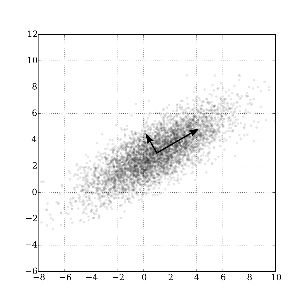
Moving forward now to 1902, Pearson noticed that even in datasets with many dimensions, a handful of principal components captured the main "drift" of the data. For example, in the data shown at right, simply looking left-to-right or up-to-down (along the original axes) might not capture the overall direction or main variation in the data. Instead, Pearson's PCA (principal component analysis) finds a new, synthesized dimension. This single synthesized dimension (see the big arrow, at right) is often the best way to model the data's primary structure
Pearson's math for PCA might make your eyes glaze over, but the core idea is pretty simple. If you want to see the "direction" of your data rows:
- Figure out a way to measure the distance between rows1.
- Draw a line between two rows that are super far apart, let's call them A and B.
- Draw a second line at a right angle to that first one.
- Plot every other data point based on where it lands relative to these two lines2.
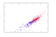
Check out this analysis on a spreadsheet with 20 columns and 800 rows describing software classes (think "lines of code," "number of unique symbols," etc.). The red dots are code with known bugs.
Now imagine yourself trying to understand the raw data (800 rows, 20 numbers). All you might see is a jumbled mess. But after this trick, everything lines up like soldiers on parade, with the bad-boy defective codes clearly visible on the right.
The here lesson is clear: problems, and the data they spit out, often have a simpler, hidden structure. And you can use this simplicity to your advantage.
For instance:
-
Amarel's Narrows (1960s): Back in the '60s, Amarel spotted "narrows" in search problems – tiny sets of essential variable settings. Miss these, and you're lost [11]. His trick? Create "macros" to jump between these narrows, like secret passages in a maze, speeding up the search big time.
-
Kohavi & John 's Variable Pruning (1990s): Fast forward to the '90s, Kohavi and John showed you could chuck out up to 80% of variables in some datasets and still get great classification accuracy [13]. Sound familiar? It's Amarel's idea again: focus on the VIP variables, not the whole crowd.
-
Crawford & Baker's ISAMP (1990s): Around the same time, constraint satisfaction folks found that "random search with retries" was surprisingly effective. Crawford and Baker's ISAMP tool would randomly poke around a model until it hit a dead end [12]. Instead of fussing, ISAMP would just note where it got stuck, hit reset, and try a different random path. Why did this wacky method work? They figured models have a few "master variables" (our keys!) pulling the strings. Trying to check every setting is a waste of time if only a few matter. If you're stuck, don't tiptoe – jump to a whole new area.
-
Williams et al.'s Backdoors: Williams and his colleagues found that if you run a random search enough times, the same few variable settings pop up in all good solutions [10]. Set these magic variables first, and crazy-long searches suddenly became quick and easy. They called this the "backdoor" to reducing computational complexity. Pretty tricky, right?
-
Modern Feature Selection: Today's machine learning is built on this. Techniques like LASSO regression (which shrinks less important variable coefficients, sometimes to zero) or using feature importance scores from decision trees are all about finding and focusing on those powerhouse variables.
-
Knowledge Distillation: Another cool, modern take on this is knowledge distillation. Here, a large, complex 'teacher' model (trained on tons of data) transfers its 'knowledge' to a much smaller, simpler 'student' model. The student model learns to mimic the teacher's outputs, effectively capturing the essential insights without all the bulk. It's like getting the CliffNotes version of a massive textbook, but it still aces the test.
Other work in semi-supervised learning tells us that : you don't need to obsess over all your data. Semi-supervised learners rely on a few central ideas:
- Continuity/Smoothness Assumption: Points close together probably share the same label. No big jumps in meaning for tiny data shifts.
- Cluster Assumption: Data likes to hang out in clumps. Points in the same clump likely share a label. Decision boundaries should fall in the sparse areas between clumps.
- Manifold Assumption: Your high-dimensional data often chills out on a simpler, lower-dimensional surface (the "manifold"). These assumptions basically mean your data isn't a completely random mess; it has structure.
There's also maths to back up these assumptions. The Johnson-Lindenstrauss lemma which says you can project high-D data to lower-D space while mostly preserving distances. We do not have to go into the details of that result but, long story short, it is telling us that complex data can often be approximated by a much simpler data set. For instance, Kocaguneli, Tu, Peters, and Xu et al. found they could predict GitHub issue close times, effort, and defects even after ditching labels for a whopping 80%, 91%, 97%, 98%, and even 100% (respectively) of their project data. Massive datasets with thousands of rows? Sometimes, just a few dozen samples will do the trick – maybe because software project data is full of repeating patterns or follows power laws (where a few items are hugely frequent/important, and most are rare).
So, next time you're drowning in data, remember the Great Data Toss-Away. Less can seriously be more.
-
According to instance-based reasoning guru David Aha, the distance between two points A,B is \(\sum_i(D(A_i,B_i)^2)^{0.5}\) (calculated over all the independent x columns). For symbolic columns, \(D(x,y) = x!=y\). For numerics, \(D(x,y)=abs(x′−y′)\) where x' is x normalized 0..1 min..max. For missing values, assume maximum distances. For example, if x,y are both missing, then D=1. If one is missing then we make the assumption that maximizes the distance; e.g.: x=x if x!="?" else (1 if y<0.5 else 0) ↩
-
Let A,B be
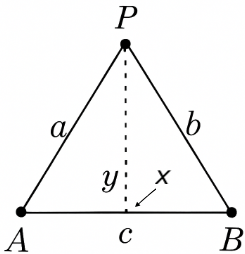 two distance points, separated by distance c. Let a point P have
a distance a,b to the points A,B. The cosine rule says P has
an x position \(x=\frac{a^2 + c^c - b^2}{2c}\) and Pythagoras
says P has a y position of \(y=(a^2-x^2)^{0.5}\). ↩
two distance points, separated by distance c. Let a point P have
a distance a,b to the points A,B. The cosine rule says P has
an x position \(x=\frac{a^2 + c^c - b^2}{2c}\) and Pythagoras
says P has a y position of \(y=(a^2-x^2)^{0.5}\). ↩
Easier AI
This book aims to show a simpler way to do many things. A repeated result is that learners learn better if they can pick their own training data. By reflecting on what has been learned so far, they can avoid the confusing, skip over the redundancies, and focus on the important parts of the data.
This technique is called active learning. And it can be extraordinary effective. For example, in software engineering (SE), systems often exhibits "funneling": i.e. despite internal complexity, software behavior converges to few outcomes, enabling simpler reasoning. Funneling explains how my imple BareLogic" active learner can build models using very little data for (e.g.) 63 SE multi-objective optimization tasks from the MOOT repository. These tasks are quite diverse and include
- software process decisions,
- optimizing configuration parameters,
- tuning learners for better analytics.
Successful for this MOOT problems results (e.g.) better advice for project managers, better control of software options, and enhanced analytics from learners that are better tuned to the local data.
MOOT includes 100,000s of examples with up to a thousand settings.
Each example is labelled with up to five effects. BareLogic's task is to find the best example(s),
after requesting the least number of labels . To do this,
BareLogic labels N=4 rest examples, then it:
- Scores and sorts labeled examples by "distance to heaven" (where "heaven" is the ideal target for optimization, e.g., weight=0, mpg=max)
- Splits the sort into
sqrt(𝑁)bestand𝑁−sqrt(𝑁)restexamples. - Trains a two-class Bayes classifier on the
bestandrestsets. - Finds the unlabeled example
Xthat is most likelybestvia
argmax(x):log(like(best|X)) - log(log(rest|X)) - Labels
X, then incrementsN. - If
X<Stopthen loop back to step1. Else returnmost(thebest[0]item) and a regression tree built from the labeled examples.
BareLogic was written for teaching purposes as a simple demonstrator of active learning. But in a result consistent with "funneling", this quick-and-dirty tool achieves near optimal results using a handful of labels. As shown by the histogram, right-hand-side of this figure, across 63 tasks:
- eight labels yielded 62% of the optimal result;
- 16 labels reached nearly 80%,
- 32 labels approached 90% optimality,
- 64 labels barely improves on 32 labels,
- etc.
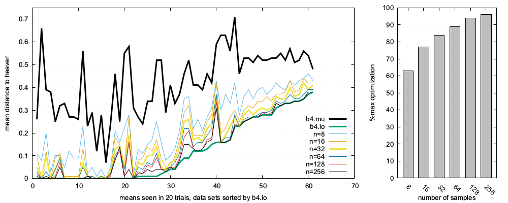 Figure: 20 runs of BareLogic on 63 multi-objective tasks.
 Histogram shows mean (1 − (most − b4.min)/(b4.mu − b4.min)). Most is the best example returned by BareLogic. b4 are the untreated examples. min is the optimal example closest to heaven.
The lesson here is that achieving state-of-the-art results can be achieved with smarter questioning, not planetary-scale computation (i.e. big AI tools like large language models, or LLMs). Active learning addresses many common concerns about AI such as slow training times, excessive energy needs, esoteric hardware requirements, testability, reproducibility, and explainability.
- The above figure was created without billions of parameters. Active learners need no vast pre-existing knowledge or massive datasets, avoiding the colossal energy and specialized hardware demands of large-scale AI.
- Further, unlike LLMs where testing is slow and often irreproducible, BareLogic's Bayesian active learning is fast (e.g., for 63 tasks and 20 repeated trials, this figure was generated in three minutes on a standard laptop).
- Most importantly, active learning fosters
human-AI partnership.
- Unlike opaque LLMs, BareLogic's results are
explainable via small labeled sets (e.g.,
N=32). Whenever a label is required, humans can understand and guide the reasoning. - The resulting tiny regression tree models offer concise, effective, and generalizable insights.
- Unlike opaque LLMs, BareLogic's results are
explainable via small labeled sets (e.g.,
Active learning provides a compelling alternative to sheer scale in AI.
- Its ability to deliver rapid, efficient, and transparent results fundamentally questions the "bigger is better" assumption dominating current thinking about AI.
- It tell us that intelligence requires more than just size.
I am not the only one proposing weight loss for AI.
- The success of LLM distillation (shrinking huge models for specific purposes) shows that giant models are not always necessary.
- Active learning pushes this idea even further, showing that leaner, smarter modeling can achieve great results.
- So why not, before we build the behemoth, try something smaller and faster?
Install the Software
To demonstrate the message of this book, we use the BareLogic tool.
What to Instakk First
| essential | what | notes |
|---|---|---|
| ✔ | bash | e.g. inside VSCode, or in googlecode, or on a terminal in Linux or Mac, or the WSL for windows |
| ✔ | a good code editor | e.g. vscode, or nvim (but consider the merits of something very lightweight like micro) |
| ✔ | Python | version 3.13 (or later) |
| ✔ | Git | |
| ✔ | Gawk | or awk, version 5 or later |
| ❌ | htop | or some other cpu minitor |
| ❌ | plylint | or some other static linter |
| ❌ | docco | or some other simple documentation generator |
Install code and data sets
Now you need some code and sample data sets
-
In a new directory, chack out our test data
mkdir newDir # call it anything you like cd newDir git clone http://github.com/timm/moot # do not change directories. Goto step 1 -
Go to https://github.com/timm/barelogic and click the Fork button.
-
Clone your fork to your local machine:
git clone https://github.com/timm/barelogic.git cd barelogic -
Fetch all branches and check out the
v0.6branch:git fetch origin git checkout -b v0.6 origin/v0.6 -
Create a new branch for your changes.
git checkout -b my-feature -
Test your install (see below)
-
Now you can start working. Make your edits in this directory. Frequently, push your changes to your on-line repo
git add . # add waht ever is new
git commit -m "Describe your changes"
git push origin my-feature
Test your install
Are you running Python3?
python3 --version
You should see Python 3.13 (or higher).
Is your data in the right place?
cd barelogic/src
make stats
If this works, you should see something like this:
    x      y   rows
------ ------ ------
     3      1    197 ../../moot/optimize/config/wc+rs-3d-c4-obj1.csv
     3      1    197 ../../moot/optimize/config/wc+sol-3d-c4-obj1.csv
     3      1    197 ../../moot/optimize/config/wc+wc-3d-c4-obj1.csv
...
If this test fails, check you have installed gawk and that the data is in the right place; i.e. from the src directory, ../../moot/optimize
Is your active learner working?
cd barelogic/src
python3 -B bl.py --quick | column -s, -t
This will run an experiments. 30 times it will run the active learner using 8,16,20,30,40 samples, then statistically compare
the results. Best results will be marked with an a; second best b. and so on.
#['rows'   'lo'     'x'   'y'   'ms'   'b4'        40          20          16          8           'name']
[398       '0.17'   4     3     5      'c 0.56 '   'a 0.17 '   'a 0.21 '   'a 0.24 '   'b 0.26 '   'auto93']
Notice that everything is "a" from 16 samples and up. This is to say that there was no win here above 16 sampples.
Is your tree learner working?
cd barelogic/src
python3 -B bl.py --tree
This test does the active learning (with 32 samples) then builds a tree from the labeled data.
auto93.csv
o{:mu1 0.556 :mu2 0.265 :sd1 0.162 :sd2 0.064}
 d2h  win    n
---- ---- ----
0.50   -4   32
0.43   13   27    Volume <= 350
0.39   25   19    |  Model >  80
0.30   45    2    |  |  origin == 2 ;
0.36   31   13    |  |  origin == 3
0.29   49    2    |  |  |  Volume <= 85 ;
0.37   28   11    |  |  |  Volume >  85
0.36   31    7    |  |  |  |  Volume <= 91
0.36   31    5    |  |  |  |  |  Model >  81 ;
0.36   30    2    |  |  |  |  |  Model <= 81 ;
0.39   23    4    |  |  |  |  Volume >  91
0.39   24    2    |  |  |  |  |  Volume <= 107 ;
0.40   21    2    |  |  |  |  |  Volume >  107 ;
0.52   -8    4    |  |  origin == 1
0.44   12    2    |  |  |  Volume >  232 ;
0.60  -28    2    |  |  |  Volume <= 232 ;
0.55  -15    8    |  Model <= 80
0.52   -8    6    |  |  Volume <= 119
0.43   13    3    |  |  |  Clndrs >  3 ;
0.60  -28    3    |  |  |  Clndrs <= 3 ;
0.64  -38    2    |  |  Volume >  119 ;
0.86  -92    5    Volume >  350
0.84  -88    2    |  Volume <= 440 ;
0.87  -95    3    |  Volume >  440 ;
Here:
nis the number of rows in each branch;;denotes a leaf;d2his the distance of the mean score of the rows in each branch to an optimal zero point (so lower numbers are better)winnormalizes d2h as100 - 100 * int(1 - (d2h-min)/(mu-min))(so higher numbers are better and 100 is best).
Is your tree learner working, on all data sets?
cd barelogic/src
time make trees
This will run the active learner (with 32 samples), then the tree learner, on all data sets. On my machine (with 10 coy cores) this takes under a minute. The thing to check here is that there are no crashes.
How good are those trees?
This final test will launch 250 Python processes. So shut down everytime else you are doing before trying this. And it freezes your computer, just do a reboot.
cd barelogic/src
time make aftersReport
This takes five minutes to run n my 10 core machine. If it works, then it prints a little report showing how good are the trees learned from 2,30,40,50 samples (selected by active learning) at selecting for good examples in the unlabeled space.
In that second round sampling, if you all 20 additional samples then:
samples + additional 10 30 50  70  90
-------   ---------- -- -- -- --- ---
     50     20       67 94 98 100 100
     40     20       70 91 97 100 100
     30     20       71 89 96 100 100
     20     20       72 86 95 100 100

    256      1      -14 33 68  78  92
    128      1       22 56 71  85  97
     64      1       12 55 70  79  95
     32      1       15 43 56  76  95
     16      1      110 31 46  67  89
      8      1        7 15 28  38  58
This report says that (say) after 64 initial samples, the 1 more from the tree, these tries select for examples in the unlabeled space that are 70% (median) of the way to optimal. Which is pretty amazing.
Further, in terms of predicting future labels, there is little win after 64 initial samples.
Pull requests
If you do something really cool, or if you fix a bug in my code, I will ask you for a pull request
- On GitHub, go to your fork and click "Compare & pull request".
- Set the pull request’s base to
timm/barelogic, branchv0.5, and compare it withYOUR_USERNAME/my-feature. - Add a descriptive title and message, then click "Create pull request".
Tutorial: Using bl.py for Multi-Objective Reasoning & Active Learning
This tutorial explains how to use the bl.py script for finding "good" solutions in your data when you have multiple, possibly conflicting, goals. We'll also see how active learning helps achieve this by looking at very few examples. We'll use the auto93.csv dataset, which is about cars.
1. The Goal: Finding the "Best" Cars with Multiple Objectives
Imagine you're looking for a car. You probably don't want just any car. You want one that's good in several ways:
- Low weight (
Lbs-inauto93.csv) - Good acceleration (
Acc+) - High miles per gallon (
Mpg+)
The challenge is that these goals often conflict. A super lightweight car might not be the fastest, and a fuel-efficient car might have slower acceleration. This is where multi-objective reasoning comes in: finding items that offer the best overall balance or trade-off across these different criteria.
The bl.py script helps with this by looking at how you've named your columns in the CSV file. A - at the end means "minimize this," and a + means "maximize this."
2. How bl.py Measures "Goodness": The ydist Function
To compare different cars, bl.py needs a single score that summarizes how well a car meets all your objectives. This is done by an aggregation function called ydist.
Here's how ydist works conceptually:
- Normalization: It takes values from different scales (like weight in pounds and MPG) and converts them to a common 0-to-1 scale.
- Distance from Ideal: For each of your goals (e.g.,
Lbs-,Acc+,Mpg+), it measures how far the car's normalized value is from the "perfect" score (0 for minimization goals likeLbs-, and 1 for maximization goals likeAcc+andMpg+). - Combined Score: It then combines these individual "distances from ideal" into one overall
ydistscore. A lowerydistis better, indicating the car is closer to the ideal across all your stated objectives.
To see this in action, you can run bl.py with an example command that processes your data and shows these distances. The eg-data command will load a CSV and print statistics for each column, including objective columns which are the basis for ydist.
python bl.py --data -f data/auto93.csv
This command processes auto93.csv and shows, among other things, the characteristics of the objective columns (y columns) from which ydist is calculated. While it doesn't directly output the ydist for each row via cthis specific command, the script contains eg-ydist (run via test/ydata.py) that does show this.
Illustrative Output (Conceptual, if eg-ydist were run, showing best and worst):
Clndrs  Volume  HpX  Model  origin  Lbs-  Acc+  Mpg+  ydist
------  ------  ---  -----  ------  ----  ----  ----  -----
4       90      48   80     2       2085  21.7  40    0.17
4       91      67   80     3       1850  13.8  40    0.17
4       86      65   80     3       2019  16.4  40    0.17
4       86      64   81     1       1875  16.4  40    0.18
...
8       429     198  70     1       4341  10.0  20    0.77
8       350     165  70     1       3693  11.5  20    0.77
8       455     225  70     1       4425  10.0  10    0.77
8       454     220  70     1       4354  9.0   10    0.79
Active Learning: Smarter Searching, Fewer Labels with actLearn
Manually checking every single car in a large dataset (i.e., "labeling" it with its performance metrics) can be very time-consuming or expensive. Active learning is a technique to find the best items by looking at only a small, intelligently chosen subset of the data.
bl.py uses the actLearn function for this. Here's the core idea:
- Tiny Start: It begins by evaluating a very small number of randomly selected cars (e.g., 4 cars, controlled by the
-sor--startflag). - Learn and Query: Based on what it learns from these initial cars, it decides which unlabeled car would be most informative to evaluate next. It does this by:
- Maintaining a small set of the
bestcars found so far and arestset. - For new candidate cars, it calculates how
likely they are to belong to the ibestset versus therestset (using a simplified Naive Bayes approach). - It then uses an "acquisition strategy" (set by
-aor--acq, e.g.,xploitto focus on known good areas,xploreto investigate uncertain areas) to pick the next car to "label" (i.e., calculate itsydist). Iterate: It repeats this process, adding the newly evaluated car to its knowledge, and refining its understanding of what makes a "good" car. Stop: It continues until it has evaluated a pre-set small number of cars (e.g., 32 by default, controlled by-Sor--Stop).
The goal of actLearn is to identify a high-quality set of cars using far fewer evaluations than if you checked every single one.
Running an Active Learning Experiment:
You can simulate this process using the --actLearn
command-line flag (which, internally, calles the `eg__actLearn`` function)
and. This will run the active learning strategy and report on how well it performed.
python bl.py --actLearn -f data/auto93.csv -S 32
Interpreting the Output from eg-actLearn:
The script will output an "object" (a summary of results). Key things to look for:
- win: A score (ideally close to 1.0) indicating how close the best car found by actLearn is to the true best car in the entire dataset (if it were known). A higher "win" means active learning did a good job.
- mu1: The ydist score of the best car found by actLearn. lo0, mu0, hi0: These show the minimum, average, and maximum ydist if all cars were evaluated. This gives you a baseline to compare mu1 against.
- stop: The number of cars actLearn actually "labeled" or evaluated (e.g., 32).
- ms: The average time in milliseconds per run.
An example output might look like:
o{:win 0.87, :rows 398, :x 4, :y 3, :lo0 0.17, :mu0 0.56, :hi0 0.93, :mu1 0.22, :sd1 0.06, :ms 5, :stop 32, :name auto93}
This (hypothetical) output would mean that by only looking at 32 cars, actLearn found a car with a ydist of 0.22. This is 87% of the way from the average car's score (0.56) towards the best possible score in the dataset (0.17). This demonstrates finding a very good solution with minimal labeling effort.
Why "Bare Logic"?
bl.py is termed "bare logic" because it implements these AI concepts (data handling, normalization, distance metrics, a simplified Bayesian approach for active learning) from fundamental principles. It avoids large external machine learning libraries, which makes the code:
- Transparent: Easier to see how calculations are done.
- Lightweight: Minimal dependencies.
- Educational: Good for understanding the core mechanics.
To Experiment Further:
- Use the -f flag with python bl.py [example_function] to specify your own CSV data file. For example, python bl.py --actLearn -f path/to/your/data.csv.
- Change the -s (start evaluations) and -S (total evaluations) flags to see how performance changes with more or fewer labels. E.g., python bl.py --actLearn -s 10 -S 50.
- Test different active learning strategies with the -a flag (e.g., python bl.py --actLearn -a xplore).
- Explore other eg-* functions by running python bl.py -h to see what else the script can do. (Note: The example functions are prefixed with eg_ in the code, so on the command line, you'd use --functionName).
By using bl.py and its command-line flags, you can perform sophisticated multi-objective reasoning and leverage active learning to find good solutions efficiently, even when data labeling is a constraint.
References
A
Aha,1991
Aha, D.W., Kibler, D. & Albert, M.K. Instance-based learning algorithms. Mach Learn 6, 37–66 (1991). https://doi.org/10.1007/BF00153759
Amarel,1960s
S. Amarel, "Program Synthesis as a Theory Formation Task: Problem Representations and Solution Methods" in Machine Learning: An Artificial Intelligence Approach: Volume II, Morgan Kaufmann, pp. 499-569, 1986. THis paper, written in the 1960s, was reprinted in this collection.
C
Chapelle,2006
Chapelle, Olivier, Bernhard Scholkopf, and Alexander Zien. "Semi-supervised learning (chapelle, o. et al., eds.; 2006)[book reviews]." IEEE Transactions on Neural Networks 20.3 (2009): 542-542.
Columbia,2003
Columbia Accident Investigation Board (CAIB). (2003). Report Volume I. National Aeronautics and Space Administration.
Crawford,1994
J. Crawford and A. Baker, "Experimental Results on the Application of Satisfiability Algorithms to Scheduling Problems", Proc. American Assoc. Artificial Intelligence (AAAI 94), pp. 1092-1097, 1994.
F
Fisher,2012
Danyel Fisher, Rob DeLine, Mary Czerwinski, and Steven Drucker. 2012. Interactions with big data analytics. interactions 19, 3 (May + June 2012), 50–59. https://doi.org/10.1145/2168931.2168943
Fu,2017
Fu, W., Menzies (2017). Easy over Hard: A Case Study on Deep Learning, In Proceedings of the 2017 11th Joint Meeting on Foundations of Software Engineering (ESEC/FSE 2017). Association for Computing Machinery, New York, NY, USA, 49–60. https://doi.org/10.1145/3106237.3106256
H
Hindle,2012
A. Hindle, E. T. Barr, Z. Su, M. Gabel, and P. Devanbu, “On the naturalness of software,” in Proc. 34th Int. Conf. Softw. Eng. (ICSE), Piscataway, NJ, USA: IEEE Press, 2012, pp. 837–847.
Hou,2024
C. Hou, Y. Zhao, Y. Liu, Z. Yang, K. Wang, and et al. 2024. Large Language Models for SE: A Systematic Literature Review. TOSEM 33, 8 (Sept. 2024).
Hutson,2018
Matthew Hutson , Artificial intelligence faces reproducibility crisis. Science 359, 725-726 (2018).DOI:10.1126/science.359.6377.725
J
Johnson,1984
W. B. Johnson and J. Lindenstrauss, “Extensions of lipschitz mappings into a hilbert space,” Contemporary Math., vol. 26, pp. 189–206, 1984.
K
Kocaguneli,2013
E. Kocaguneli, T. Menzies, J. Keung, D. Cok, and R. Madachy, “Active learning and effort estimation: Finding the essential content of software effort estimation data,” IEEE Trans. Softw. Eng., vol. 39, no. 8, pp. 1040–1053, Aug.2013.
Kohavi,1997
R. Kohavi and G. H. John, "Wrappers for Feature Subset Selection", Artificial Intelligence, vol. 97, no. 1–2, pp. 273-324, 1997.
L
Lin,2015
Z. Lin and J. Whitehead, “Why power laws? An explanation from fine-grained code changes,” in Proc. IEEE/ACM 12th Work. Conf. Mining Softw. Repositories, Piscataway, NJ, USA: IEEE Press, 2015, pp. 68–75.
Lustosa,2025
A. Lustosa and T. Menzies. 2025. Less Noise, More Signal: DRR for Better Optimizations of SE Tasks arXiv:2503.21086 https://arxiv.org/abs/2503.21086
M
Majumder,2018
Majumder, S., Balaji, N., Brey, K., Fu, W., & Menzies, T. (2018). 500+ times faster than deep learning. In Proceedings of the 15th International Conference on Mining Software Repositories. ACM.
Menzies,2007a
T. Menzies, D. Owen, and J. Richardson. 2007. The Strangest Thing About Software Computer 40, 1 (2007), 54–60.
Menzies,BL
T. Menzies. 2025. BareLogic Python Source Code. https://github.com/timm/ barelogic/blob/main/src/bl.py.
Menzies,MOOT
T. Menzies. 2025. MOOT= Many multi-objective optimization tests. https://github. com/timm/moot/tree/master/optimize.
Menzies,2008
T. Menzies, B. Turhan, A. Bener, G. Gay, B. Cukic, and Y. Jiang, “Implications of ceiling effects in defect predictors,” in Proc. 4th Int. Workshop Predictor Models Softw. Eng., 2008, pp. 47–54.
Menzies,2025a
"Retrospective: Data Mining Static Code Attributes to Learn Defect Predictors" in IEEE Transactions on Software Engineering, vol. 51, no. 03, pp. 858-863, March 2025, doi: 10.1109/TSE.2025.3537406.
N
Nair,2018
Nair, V., Menzies, T., Siegmund, N., & Apel, S. (2018). Using bad learners to find good configurations. Proceedings of the 2018 26th ACM Joint Meeting on European Software Engineering Conference and Symposium on the Foundations of Software Engineering, 448-459.
O
Ostrand,2004
Thomas J. Ostrand, Elaine J. Weyuker, and Robert M. Bell. 2004. Where the bugs are. SIGSOFT Softw. Eng. Notes 29, 4 (July 2004), 86–96. https://doi.org/10.1145/1013886.1007524
P
Pearson,1902
Pearson, K. (1902). On Lines and Planes of Closest Fit to Systems of Points in Space. Philosophical Magazine, 6(2), 559-572. https://doi.org/10.1080/14786440209478072
Peters,2015
F. Peters, T. Menzies, and L. Layman, “Lace2: Better privacy-preserving data sharing for cross project defect prediction,” in Proc. IEEE/ACM 37th IEEE Int. Conf. Softw. Eng., vol. 1, 2015, pp. 801–811.
S
Settles,2009
D. Settles. 2009. Active learning literature survey. Technical Report 1648. U. Wisconsin-Madison Dept of CS.
Strubell,2018
Strubell, E., Ganesh, A., & McCallum, A. (2019). Energy and Policy Considerations for Deep Learning in NLP. Proceedings of the 57th Annual Meeting of the Association for Computational Linguistics, 3645-3650.
T
Tawosi,2023
V. Tawosi, R. Moussa, and F. Sarro. 2023. Agile Effort Estimation: Have We Solved the Problem Yet? IEEE Trans SE 49, 4 (2023), 2677–2697.
Tu,2022
H. Tu and T. Menzies, “Frugal: unlocking semi-supervised learning for software analytics,” in Proc. ASE, Piscataway, NJ, USA: IEEE Press, 2022, pp. 394–406.
V
Van Engelen,2020
Van Engelen, Jesper E., and Holger H. Hoos. "A survey on semi-supervised learning." Machine learning 109.2 (2020): 373-440.
W
Williams,2002
R. Williams, C. P. Gomes and B. Selman, "Backdoors to Typical Case Complexity", Proc. IJCAI, 2003, [online] Available: www.cs.cornell.edu/gomes/papers/backdoors.pdf.
X
Xu,2015
Tianyin Xu, Long Jin, Xuepeng Fan, Yuanyuan Zhou, Shankar Pasupathy, and Rukma Talwadker. 2015. Hey, you have given me too many knobs!: understanding and dealing with over-designed configuration in system software. In Proceedings of the 2015 10th Joint Meeting on Foundations of Software Engineering (ESEC/FSE 2015). Association for Computing Machinery, New York, NY, USA, 307–319. https://doi.org/10.1145/2786805.2786852
Xu,2021
Z. Xu , “A comprehensive comparative study of clustering-based unsupervised defect prediction models,” J. Syst. Softw., vol. 172, 2021, Art. no. 110862.
Z
Zeming,2024
L. Zeming and et al. 2024. A Survey on Knowledge Distillation for Large Language Models. ACM Trans. Int. Systems & Technology (2024).